Observability Analytics lets you visualize [SQL](https://docs.cloud.google.com/bigquery/docs/reference/standard-sql/query-syntax.md.txt) query results as charts to
identify patterns and trends in your trace data. After you run a query to search
and aggregate trace data, you can view the results in a table, convert them into
a chart, and save the visualization to a dashboard.
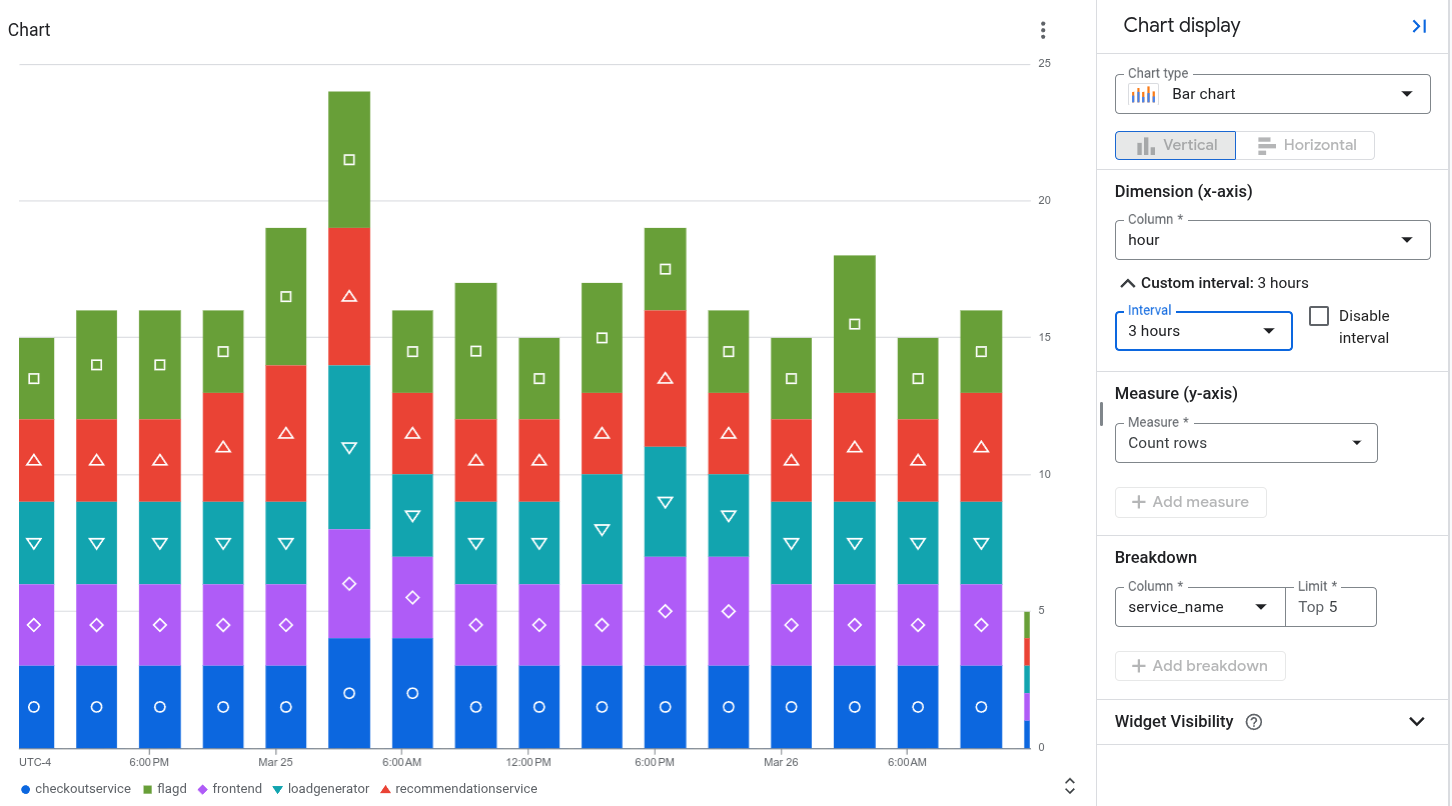
For example, the following chart displays the status reported by spans over
time, grouped by `service_name`:
## Before you begin
1.
To get the permissions that
you need to load the **Observability Analytics** page, write and run queries on
your trace data, and save charts on custom dashboards,
ask your administrator to grant you the
following IAM roles:
- [Observability View Accessor](https://docs.cloud.google.com/iam/docs/roles-permissions/observability.md.txt#observability.viewAccessor) (`roles/observability.viewAccessor`) on the observability views that you want to query. This role supports IAM conditions, which let you restrict the grant to a specific view. If you don't attach a condition to the role grant, then the principal can access all observability views.
- [Monitoring Editor](https://docs.cloud.google.com/iam/docs/roles-permissions/monitoring.md.txt#monitoring.editor) (`roles/monitoring.editor`) on your project.
For more information about granting roles, see [Manage access to projects, folders, and organizations](https://docs.cloud.google.com/iam/docs/granting-changing-revoking-access.md.txt).
You might also be able to get
the required permissions through [custom
roles](https://docs.cloud.google.com/iam/docs/creating-custom-roles) or other [predefined
roles](https://docs.cloud.google.com/iam/docs/roles-overview#predefined).
## Select the data to chart
To configure what data to display on a chart, build a query by using
[SQL](https://docs.cloud.google.com/bigquery/docs/reference/standard-sql/query-syntax.md.txt).
When you select the **Chart** tab, a chart displays your query
results. After you run the query and generate a chart, you can
customize the chart by changing the chart type and selecting
columns to display different data.
To view your query results as a chart, run a query by doing the following:
1. In the Google Cloud console, go to the
**Observability Analytics** page:
[Go to **Observability Analytics**](https://console.cloud.google.com/logs/analytics)
If you use the search bar to find this page, then select the result whose subheading is
**Logging**.
2. In the **Query** pane, enter a query and then click **Run**.
3. After the query has completed, in the **Results** tab, select how you want
to view your query results:
- **Table**: Tabular format only.
- **Chart**: Chart format only.
- **Both**: Chart and tabular format.
After you select how to view your query results, you can configure any
fields for the selected visualization, and then save the query and results
to a custom dashboard. The saved format is tabular when you've selected
the **Table** option. Otherwise, the format is a chart.
For charts, the visualization options let you select the chart type,
and select which rows and columns are charted. For more information
about the chart configuration, see
[Customize chart configuration](https://docs.cloud.google.com/trace/docs/analytics-chart.md.txt#chart-config).
## Customize chart configuration
You can customize the chart configuration by changing the chart type, selecting
the dimension and measure to chart, and by applying a breakdown. The
**Dimension** is used to group or categorize rows and is the X-axis value. The
**Measure**, or the Y-axis value, is a data series that is plotted against the
Y-axis.
### Change chart type
You can select from the following chart types, depending on what kind of rows
and columns you selected as the dimension and measure, and how you want that
data to be visualized.
- Bar chart (default):
Bar charts plot data on two axes. If your chart uses a category or string
as the dimension, then you can set the chart configuration for a bar chart to
horizontal or vertical, where the dimension and measure axes are swapped.
- Line chart:
Line charts can be used to show data changes over time. When you use a line
chart, each time series is shown by a different line that corresponds to
the measure(s) you have selected.
If your X-axis is time-based, each data point is placed at the beginning of
a time interval. Each data point is connected by linear interpolation.
- Stacked area chart:
An area chart is based on a line chart, and the area below each line is
shaded. In area charts, the data series are stacked. For example, if you have
two identical series, then the series overlap in a line chart, but the
shaded area is stacked in an area chart.
- Pie or donut chart:
A pie chart shows how categories in a dataset relate to the whole dataset,
by using a circle to represent the whole dataset and wedges in the circle
to represent the categories in the dataset. The size of a wedge
indicates how much, often as a percentage, the category contributes to
the whole.
- Table:
A table shows one row for each row in the query result. The columns in the
table are defined by the `SELECT` clause. If you plan to display data
in tabular form on a dashboard, then use a `LIMIT` clause to restrict the
number of rows in the result to be less than a few hundred.
- Gauge or scorecard:
Gauges and scorecards provide you with the most recent value along with
a green, amber, or red indication
based on how that value compares to a set of thresholds.
Unlike gauges, which only show information about the most recent
value, scorecards can also include information about past values.
Gauges and scorecards can only display the query result when the query
result contains at least one row, and that row contains a column with a
timestamp and a column with numeric data. The query result can contain
multiple rows and more than two columns.
If you want to perform the time-based aggregation as part of your query,
then do the following:
- Configure your query to aggregate data over a time interval, to order
the results by descending timestamps, and to limit the number of
rows in the results. You can use the `LIMIT` clause or use the
time range selector to limit the number of rows in the query result.
For example, the following queries your trace data, and it aggregates
the data over one-hour intervals, applies a limit, and sorts the
results:
```sql
SELECT TIMESTAMP_TRUNC(start_time, HOUR) AS hour,
COALESCE(
JSON_VALUE(resource.attributes, '$."service.name"'),
JSON_VALUE(attributes, '$."service.name"'),
JSON_VALUE(attributes, '$."g.co/gae/app/module"')) AS service_name,
status.code AS status,
COUNT(*) AS count
FROM `PROJECT_ID.LOCATION._Trace.Spans._AllSpans`
GROUP BY hour, service_name, status
ORDER BY hour DESC
LIMIT 1000
```
The following describes the meaning of the fields in the previous
expression:
- PROJECT_ID: The identifier of the project.
- LOCATION: The [location of the observability bucket](https://docs.cloud.google.com/stackdriver/docs/observability/observability-bucket-locations.md.txt).
The previous query was used to generate the figure shown at the
beginning of this document. That figure also shows the chart
configuration.
- Set the **Dimension** to match the column that reports the time-unit.
For example, if your query aggregates data by one hour and creates a
column named `hour`, then set the **Dimension** menu to `hour`.
- Select **Disable interval** because your query already specifies the
aggregation interval. In the example, this interval is one hour.
- Set the **Measure** to the numeric column, and set the function to
**none**.
> [!NOTE]
> **Note:** If your query performs time-based aggregation, then make sure that you follow the previous guidance. Other settings result in both your query and Observability Analytics performing aggregation operations, which results in the gauge or scorecard displaying unexpected values.
If you want to rely on Observability Analytics to perform the time-based aggregation for
you, then do the following:
- Configure the time-range selector, which affects the number of rows in the query result.
- Set the **Dimension** to match the column that reports the time-unit. For example, you might set this menu to `timestamp`.
- Set the **Interval** menu to a specific aggregation interval. For example, set the value of this field to `1 hour`. Don't select **Automatic interval**.
- Set the **Measure** to the numeric column, and select a function such as **sum**.
### Change dimension and measure
You can choose which rows and columns are charted by selecting the dimension
and measure fields.
> [!NOTE]
> **Note:** If your query results contain a column that has long strings, such as error messages, and you select that column to be the dimension or breakdown, then your chart might have errors or unexpected values.
- Dimension
The dimension must be a timestamp, numeric, or string column. By default, the dimension is set to
the first timestamp-based column in the schema. If no timestamp is present in the query, then the
first string column is selected as the dimension. You can also customize what the dimension is in
the **Chart display** panel. When a timestamp column is selected as the dimension, then the chart
shows how data changes over time. When a string column is selected as the dimension for a bar chart,
you can sort the data by ascending or descending, which sorts the dimension by lexical order. You
can also keep the \`default\` sort order, which sorts the dimension based on the values of the
corresponding measure in descending order.
By default, the interval for timestamps is automatically
set, but you can also select a custom interval. Automatic intervals change
values based on the time-range selector to maintain similarly sized groups.
You can also disable the interval, which lets you specify your own
aggregations and time ranges within the query for more complex analysis.
Disabling the interval sets the aggregation function of the measures
to `none`. Only numeric measures are permitted when the dimension interval
is disabled.
> [!NOTE]
> **Note:** Only the `TIMESTAMP` column can be used as a timestamp dimension. To use `DATE` and `DATETIME`, you must use the [`CAST()`](https://docs.cloud.google.com/bigquery/docs/reference/standard-sql/conversion_functions.md.txt#cast) function to convert the data types to `TIMESTAMP`.
- Measure
You can select multiple measures in the **Chart display** panel. When you select a measure, you
must also select the aggregation function to perform on its grouped values, such as
`count`, `sum`, `average`, and `percentile-99`.
For example, `count-distinct` returns the number of unique values in a given column.
If you select the **Disable interval** checkbox for the dimension, then the
`none` aggregation function option is available. If the dimension is a
string value, the **Disable interval** checkbox is not shown. However,
setting a measure's aggregation functions to `none` also disables the
interval.
### Add a breakdown
> [!NOTE]
> **Note:** If your chart contains more than one measure, then you can't add a breakdown.
To split a single data series into multiple data series based on another column, add a breakdown.
When you select a breakdown, choose columns that contain a small
number of short and meaningful labels, like `region_name`. Don't select fields
that might contain a large number of strings or long strings, like
`textPayload`.
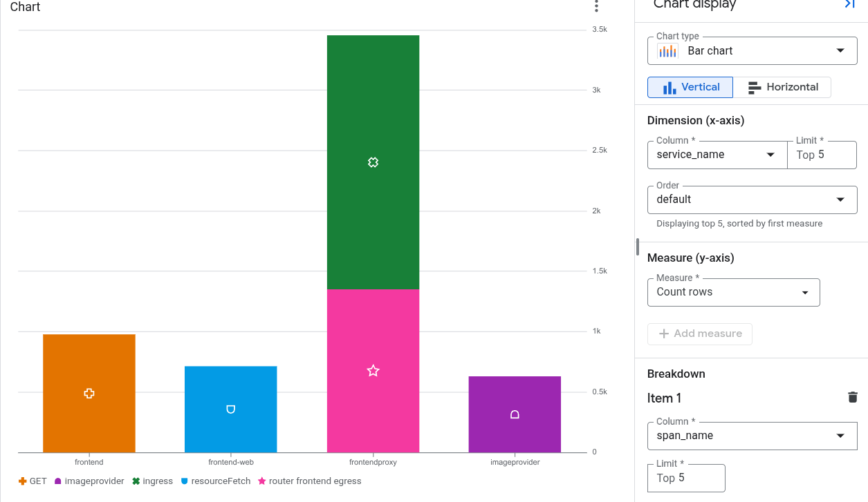
For example, the following chart displays the number of spans created by
each service, along with the data broken down by the span name:
### Generate and display trace exemplars
> [!WARNING]
>
> **Preview**
>
>
> This product or feature is
>
> subject to the "Pre-GA Offerings Terms" in the General Service Terms section
> of the [Service Specific
> Terms](https://docs.cloud.google.com/terms/service-terms#1).
>
> Pre-GA products and features are available "as is" and might have limited support.
>
> For more information, see the
> [launch stage descriptions](https://cloud.google.com/products/#product-launch-stages).
You can configure your SQL-based charts that analyze trace data to display
dynamically generated exemplars. An *exemplar* is a representative sample request
or span associated with a metric measurement. Each exemplar links to a trace;
selecting an exemplar opens a flyout that displays the trace.
#### Configuration requirements
To display exemplars, the following must be true:
- The chart's query is written in SQL and the query target is trace data.
- The chart uses the line or bar chart visualization.
- The `trace_id` and the `start_time` are part of the query results.
To hide exemplars, go to the chart's toolbar and select
**Hide exemplars**.
#### How the system generates exemplars
The system applies an intelligent sampling selection strategy to keep
exemplars readable and relevant:
- **For statistical measures such as `AVG` and `PERCENTILE`:** The system compares raw span values against the chart's interpolated trendline and groups samples into deviation pools. A proportional sample from each pool is plotted and spaced evenly over time.
- **For frequency counts such as `COUNT`:** The system positions exemplars along the upper boundary of the chart window and spaces them evenly across time and data series breakdowns.
#### Limitations
- If a chart displays multiple time series, then the system reduces the number of exemplars that are shown.
- Exemplars might not be evenly distributed in the time interval of the chart.
- The Y-axis scale might distort the visual display. Distortion is most likely when a chart uses a logarithmic Y-axis or when time series contain outliers.
- You can't configure how the system generates exemplars.
## Save a chart to a custom dashboard
After a chart is generated from your query, you can save that chart to a
[custom dashboard](https://docs.cloud.google.com/monitoring/charts/dashboards.md.txt). Custom dashboards let you
display and organize information that is useful to you by using a variety of
widget types. These dashboards also let you define variables, which are
dashboard-level filters that apply only to specific widgets. To apply a
variable to a widget, you must modify the query. For more information, see
[Apply a variable to a widget](https://docs.cloud.google.com/monitoring/dashboards/filter-permanent.md.txt#apply-permanent-filter).
A dashboard displays a warning message for a widget that contains a SQL query
when the query runs on the BigQuery engine and the queried
resources aren't in the same ownership boundary. Ownership boundaries are
determined by several factors, one of which is the hierarchy of
the resources the query uses. To prevent these warnings,
[set up a service perimeter](https://docs.cloud.google.com/vpc-service-controls/docs/set-up-service-perimeter.md.txt).
To save your chart to a dashboard, do the following:
1. In the Google Cloud console, go to the
**Observability Analytics** page:
[Go to **Observability Analytics**](https://console.cloud.google.com/logs/analytics)
If you use the search bar to find this page, then select the result whose subheading is
**Logging**.
2. Run a query to generate a chart, then click
**Save to dashboard**.
3. In the **Save to dashboard** dialog, enter a title for your chart and
select the dashboard where you want to save the chart.
4. Optional: To view the custom dashboard, in the toast,
click **View dashboard**.
To view a list of custom dashboards that contain charts generated by
SQL queries, go to the **Save to dashboard** button and click
**Menu**.
### Edit a chart saved to a custom dashboard
You can modify a chart after it has been saved to a dashboard. For more
information, see
[Modify a widget's configuration](https://docs.cloud.google.com/monitoring/charts/manage-widgets.md.txt#editing).
In the **Configure widget** dialog, you can do the following:
- Change the data you query.
- Edit the query that is used to generate a chart.
- Customize the chart configuration to visualize different data.
## Limitations
- If your Google Cloud project is in a folder that uses Assured Workloads,
then the charts that you generate can't be displayed on a custom dashboard.
- Dashboard-level filters don't apply to charts generated from a SQL query.
- Selected columns must have at least one row with a non-null value.
- If you save a query and customize the chart configuration, then the custom
chart configuration is not saved.
- If your query already contains aggregations, then the generated chart might
be different due to additional aggregation that is automatically applied
by Observability Analytics.
- JSON paths must be cast to strings or numbers in order to be charted.
## What's next
- [Save and share a SQL query](https://docs.cloud.google.com/trace/docs/analytics-save-share-query.md.txt)
- [Sample SQL queries](https://docs.cloud.google.com/trace/docs/analytics-samples.md.txt)
- [Query a linked BigQuery dataset in BigQuery](https://docs.cloud.google.com/trace/docs/analytics-query-linked-dataset.md.txt)